Gene set analysis • rvat

# Libraries
library(rvat)
library(rvatData)

Some output will be written during the tutorials, please change outdir, defined below to your preferred directory:

outdir <- tempdir()

Getting started

Load set of example rare variant results

data(rvbresults)

Data formats

geneSetList

a geneSetList() is a class for storing gene sets (+ metadata) and several methods for working with them.
Gene set lists can be generated from multiple sources, currently the following formats are supported:
- GMT-format (see [MSigDB] (https://www.gsea-msigdb.org/gsea/msigdb/).
- data.frame
- list

Generating a geneSetList object

The buildGeneSet() function can be used to load in data from one of the formats described above. For example, below we build a genesetlist based on a MSigDB GMT file including Gene Ontology (molecular function) terms:

## Build a geneSetList from a gmt-file
genesetlist <- buildGeneSet(gmtpath = "data/c5.go.mf.v2023.2.Hs.symbols.gmt")

# Check genesets:
genesetlist

## geneSetList
## Contains 1799 sets

head(names(genesetlist))

## [1] "GOMF_1_4_ALPHA_OLIGOGLUCAN_PHOSPHORYLASE_ACTIVITY"             
## [2] "GOMF_1_ACYLGLYCEROPHOSPHOCHOLINE_O_ACYLTRANSFERASE_ACTIVITY"   
## [3] "GOMF_1_ALKYL_2_ACETYLGLYCEROPHOSPHOCHOLINE_ESTERASE_ACTIVITY"  
## [4] "GOMF_1_PHOSPHATIDYLINOSITOL_3_KINASE_ACTIVITY"                 
## [5] "GOMF_1_PHOSPHATIDYLINOSITOL_3_KINASE_REGULATOR_ACTIVITY"       
## [6] "GOMF_1_PHOSPHATIDYLINOSITOL_4_5_BISPHOSPHATE_3_KINASE_ACTIVITY"

Alternatively, custom genesets can be provided like so:

genesets_custom <-  list(
  "ALS_genes" = c("SOD1", "NEK1", "FUS"),
  "PD_genes" = c("LRRK2", "GBA", "SNCA")
)
genesetlist_custom <- buildGeneSet(
    genesets_custom
)
genesetlist_custom

## geneSetList
## Contains 2 sets

Basic usage

Some basic geneSetList methods:

length(genesetlist)

## [1] 1799

lengths(genesetlist) %>% head()

##              GOMF_1_4_ALPHA_OLIGOGLUCAN_PHOSPHORYLASE_ACTIVITY 
##                                                              5 
##    GOMF_1_ACYLGLYCEROPHOSPHOCHOLINE_O_ACYLTRANSFERASE_ACTIVITY 
##                                                              8 
##   GOMF_1_ALKYL_2_ACETYLGLYCEROPHOSPHOCHOLINE_ESTERASE_ACTIVITY 
##                                                              8 
##                  GOMF_1_PHOSPHATIDYLINOSITOL_3_KINASE_ACTIVITY 
##                                                             10 
##        GOMF_1_PHOSPHATIDYLINOSITOL_3_KINASE_REGULATOR_ACTIVITY 
##                                                             16 
## GOMF_1_PHOSPHATIDYLINOSITOL_4_5_BISPHOSPHATE_3_KINASE_ACTIVITY 
##                                                              7

metadata(genesetlist) %>% head()

## $rvatVersion
## [1] "0.3.1"
## 
## $source
## [1] "data/c5.go.mf.v2023.2.Hs.symbols.gmt"
## 
## $creationDate
## [1] "2025-02-12 12:48:57"

genesetlist[[2]]

## An object of class "geneSet"
## Slot "geneSetName":
## [1] "GOMF_1_ACYLGLYCEROPHOSPHOCHOLINE_O_ACYLTRANSFERASE_ACTIVITY"
## 
## Slot "units":
## [1] "LPCAT1,LPCAT2,LPCAT3,LPCAT4,MBOAT1,MBOAT2,PRDX6,TAFAZZIN"
## 
## Slot "w":
## [1] "1,1,1,1,1,1,1,1"
## 
## Slot "metadata":
## [1] "https://www.gsea-msigdb.org/gsea/msigdb/human/geneset/GOMF_1_ACYLGLYCEROPHOSPHOCHOLINE_O_ACYLTRANSFERASE_ACTIVITY"

genesetlist[1:3]

## geneSetList
## Contains 3 sets

head(as.list(genesetlist))

## $GOMF_1_4_ALPHA_OLIGOGLUCAN_PHOSPHORYLASE_ACTIVITY
## [1] "MTAP" "PYGB" "PYGL" "PYGM" "TYMP"
## 
## $GOMF_1_ACYLGLYCEROPHOSPHOCHOLINE_O_ACYLTRANSFERASE_ACTIVITY
## [1] "LPCAT1"   "LPCAT2"   "LPCAT3"   "LPCAT4"   "MBOAT1"   "MBOAT2"   "PRDX6"   
## [8] "TAFAZZIN"
## 
## $GOMF_1_ALKYL_2_ACETYLGLYCEROPHOSPHOCHOLINE_ESTERASE_ACTIVITY
## [1] "ASPG"     "LCAT"     "PAFAH1B2" "PAFAH1B3" "PAFAH2"   "PLA2G10"  "PLA2G6"  
## [8] "PLA2G7"  
## 
## $GOMF_1_PHOSPHATIDYLINOSITOL_3_KINASE_ACTIVITY
##  [1] "ATM"     "PIK3C2A" "PIK3C2B" "PIK3C2G" "PIK3C3"  "PIK3CA"  "PIK3CB" 
##  [8] "PIK3CD"  "PIK3CG"  "PIK3R3" 
## 
## $GOMF_1_PHOSPHATIDYLINOSITOL_3_KINASE_REGULATOR_ACTIVITY
##  [1] "CCKBR"   "CISH"    "P3R3URF" "PIK3R1"  "PIK3R2"  "PIK3R3"  "PIK3R5" 
##  [8] "PIK3R6"  "SLA2"    "SOCS1"   "SOCS2"   "SOCS3"   "SOCS4"   "SOCS5"  
## [15] "SOCS6"   "SOCS7"  
## 
## $GOMF_1_PHOSPHATIDYLINOSITOL_4_5_BISPHOSPHATE_3_KINASE_ACTIVITY
## [1] "IPMK"    "PIK3C2A" "PIK3CA"  "PIK3CB"  "PIK3CD"  "PIK3CG"  "PIK3R6"

The getGeneSet() method can be used to extract one or more genesets from a geneSetList:

# Extract one specific geneset:
geneset <- getGeneSet(genesetlist, 
                      geneSet = "GOMF_E_BOX_BINDING")
geneset[[1]]

## An object of class "geneSet"
## Slot "geneSetName":
## [1] "GOMF_E_BOX_BINDING"
## 
## Slot "units":
## [1] "AHR,ASCL1,ASCL2,ATOH1,ATOH7,ATOH8,BHLHA15,BHLHE22,BHLHE23,BHLHE40,BHLHE41,BMAL1,BMAL2,CIART,CLOCK,CRY1,FIGLA,GATA3,HAND2,HDAC1,HES1,HIF1A,MAX,MITF,MYBBP1A,MYC,MYF5,MYF6,MYOD1,MYOG,NEUROD1,NEUROD2,NEUROD4,NEUROD6,NEUROG1,NEUROG2,NEUROG3,NR1D1,OLIG1,OLIG2,OLIG3,PER1,PPARG,PRMT5,PTF1A,SCRT2,SCX,SNAI1,SNAI2,SREBF2,TAL1,TCF12,TCF15,TCF21,TCF3,TCF4,TFAP4,TWIST1,ZEB1"
## 
## Slot "w":
## [1] "1,1,1,1,1,1,1,1,1,1,1,1,1,1,1,1,1,1,1,1,1,1,1,1,1,1,1,1,1,1,1,1,1,1,1,1,1,1,1,1,1,1,1,1,1,1,1,1,1,1,1,1,1,1,1,1,1,1,1"
## 
## Slot "metadata":
## [1] "https://www.gsea-msigdb.org/gsea/msigdb/human/geneset/GOMF_E_BOX_BINDING"

It can also be used to retrieve gene sets that contain one or more genes of interest:

# Extract all genesets that contain SOD1:
geneset = getGeneSet(genesetlist, unit = "SOD1")
head(names(geneset))

## [1] "GOMF_ANTIOXIDANT_ACTIVITY"             
## [2] "GOMF_COPPER_ION_BINDING"               
## [3] "GOMF_GTPASE_BINDING"                   
## [4] "GOMF_OXIDOREDUCTASE_ACTIVITY"          
## [5] "GOMF_PHOSPHATASE_BINDING"              
## [6] "GOMF_PROTEIN_FOLDING_CHAPERONE_BINDING"

Specific units/genes can also be dropped from the geneSetList(), which is useful if you want to exclude top genes for gene set analysis for example:

genesetlist_noSOD1 <- dropUnits(genesetlist, unit = "SOD1")

Convert geneSetList() to a data.frame or a list:

head(as.list(genesetlist), 2)

## $GOMF_1_4_ALPHA_OLIGOGLUCAN_PHOSPHORYLASE_ACTIVITY
## [1] "MTAP" "PYGB" "PYGL" "PYGM" "TYMP"
## 
## $GOMF_1_ACYLGLYCEROPHOSPHOCHOLINE_O_ACYLTRANSFERASE_ACTIVITY
## [1] "LPCAT1"   "LPCAT2"   "LPCAT3"   "LPCAT4"   "MBOAT1"   "MBOAT2"   "PRDX6"   
## [8] "TAFAZZIN"

head(as.data.frame(genesetlist), 3)

##                                                    geneSetName
## 1            GOMF_1_4_ALPHA_OLIGOGLUCAN_PHOSPHORYLASE_ACTIVITY
## 2  GOMF_1_ACYLGLYCEROPHOSPHOCHOLINE_O_ACYLTRANSFERASE_ACTIVITY
## 3 GOMF_1_ALKYL_2_ACETYLGLYCEROPHOSPHOCHOLINE_ESTERASE_ACTIVITY
##                                                      units               w
## 1                                 MTAP,PYGB,PYGL,PYGM,TYMP       1,1,1,1,1
## 2 LPCAT1,LPCAT2,LPCAT3,LPCAT4,MBOAT1,MBOAT2,PRDX6,TAFAZZIN 1,1,1,1,1,1,1,1
## 3 ASPG,LCAT,PAFAH1B2,PAFAH1B3,PAFAH2,PLA2G10,PLA2G6,PLA2G7 1,1,1,1,1,1,1,1
##                                                                                                             metadata
## 1            https://www.gsea-msigdb.org/gsea/msigdb/human/geneset/GOMF_1_4_ALPHA_OLIGOGLUCAN_PHOSPHORYLASE_ACTIVITY
## 2  https://www.gsea-msigdb.org/gsea/msigdb/human/geneset/GOMF_1_ACYLGLYCEROPHOSPHOCHOLINE_O_ACYLTRANSFERASE_ACTIVITY
## 3 https://www.gsea-msigdb.org/gsea/msigdb/human/geneset/GOMF_1_ALKYL_2_ACETYLGLYCEROPHOSPHOCHOLINE_ESTERASE_ACTIVITY

Remapping IDs

The IDs in a geneSetList() can be remapped using the remapIDs() method to match those used in the analyses.

Below we remap the gene symbols to Ensembl IDs, based on a linker-file.

# Linker file mapping Entrez gene IDs to Ensembl IDs:
linker <- readr::read_tsv("data/Homo_sapiens.GRCh38.105.gene.txt.gz", show_col_types = FALSE)
linker <- linker[,c("gene_id", "gene_name")]

# note: the `duplicated_ids` parameter indicates what to do with IDs that map to multiple IDs 
genesetlist_remapped <- remapIDs(genesetlist, 
                                 dict = linker[,c(2,1)], 
                                 targets = unique(rvbresults$unit), 
                                 duplicate_ids = "keep_first")

## 15574/15682 IDs in the geneSetList are present in the linker file.

genesetlist_remapped[[1]]

## An object of class "geneSet"
## Slot "geneSetName":
## [1] "GOMF_1_4_ALPHA_OLIGOGLUCAN_PHOSPHORYLASE_ACTIVITY"
## 
## Slot "units":
## [1] "ENSG00000099810,ENSG00000100994,ENSG00000100504,ENSG00000068976,ENSG00000025708"
## 
## Slot "w":
## [1] "1,1,1,1,1"
## 
## Slot "metadata":
## [1] "https://www.gsea-msigdb.org/gsea/msigdb/human/geneset/GOMF_1_4_ALPHA_OLIGOGLUCAN_PHOSPHORYLASE_ACTIVITY"

geneSetFile

We have also implemented a gene set file structure (geneSetFile()) akin to a varSetFile(), from which gene sets can be loaded without loading the entire file to memory. The buildGeneSet() function can convert a file in one of the formats mentioned in geneSetList. Below we build a GO and KEGG geneSetFile():

# build a genesetfile
buildGeneSet(gmtpath = "data/c5.go.mf.v2023.2.Hs.symbols.gmt",
            output = paste0(outdir, "/genesetfile.txt.gz")
            )

# connect 
genesetfile <- geneSetFile(paste0(outdir, "/genesetfile.txt.gz"))
genesetfile

## geneSetFile
## Path: /var/folders/cl/wvc0rvjx4vd5rzt2_fhpmfth0000gp/T//RtmpArxtd0/genesetfile.txt.gz
## Sets: 1799

Extract a gene set:

# extract a geneset from a genesetfile
genesetlist <- getGeneSet(genesetfile, 
                          geneSet = c("GOMF_UBIQUITIN_LIKE_MODIFIER_ACTIVATING_ENZYME_ACTIVITY"))
listUnits(genesetlist[[1]])

##  [1] "ATG7"  "MOCS3" "NAE1"  "SAE1"  "UBA1"  "UBA2"  "UBA3"  "UBA5"  "UBA6" 
## [10] "UBA7"

Convert to a geneSetList() (i.e. load all sets):

genesetlist <- as.geneSetList(genesetfile)

Gene-set analyses

Broadly, the GSA methods implemented in RVAT can be divided into competitive and self-contained tests, where the former tests whether genes in the gene set are more associated with the phenotype than genes outside the gene set, while the latter jointly tests whether genes in the gene set are associated with the phenotype without considering genes outside the set (de Leeuw et al. 2016). Because competitive GSA tests for an enrichment relative to the genes outside the gene set, it controls for polygenicity as well as biases such as confounding and technical variability. Self-contained tests, on the other hand, are generally more powerful but may result in inflated test-statistics in case of polygenicity or residual biases in the data. See (de Leeuw et al. 2016) for a brilliant review of GSA methods.

Competitive GSA

Currently the following competitive methods are implemented:
- linear model (test = “lm”): tests whether gene set membership predicts higher gene-association scores. Allows for adjustment for covariates such as gene size and number of variants in a gene.
- hypergeometric test (test = “fisher”): tests whether the proportion of P-values below the specified threshold is greater than the proportion outside of it.

In below example, we perform competitive gene set analysis using a linear model on gene burden results:

# Adjust for the number of variants in a gene
res <- rvbresults[rvbresults$test=="firth" & 
                    rvbresults$varSetName == "ModerateImpact", ]
GSAresults <- geneSetAssoc(
  res,
  genesetlist,
  covar = c("nvar"),
  test = c("lm"), 
  minSetSize = 10,
  maxSetSize = 500
)

topResult(GSAresults)

## gsaResult with 10 rows and 11 columns
##               geneSetName  test covar threshold geneSetSize  genesObs    effect
##                     <Rle> <Rle> <Rle> <numeric>   <numeric> <numeric> <numeric>
## 1  GOMF_MRNA_METHYLTRAN..    lm  nvar        NA          13        13  0.878627
## 2        GOMF_BMP_BINDING    lm  nvar        NA          20        19  0.537316
## 3  GOMF_DYNEIN_LIGHT_IN..    lm  nvar        NA          28        28  0.419752
## 4  GOMF_DYNEIN_HEAVY_CH..    lm  nvar        NA          16        16  0.553052
## 5  GOMF_PROTEIN_KINASE_..    lm  nvar        NA          25        24  0.436416
## 6  GOMF_TRANSFERRIN_REC..    lm  nvar        NA          11        10  0.664977
## 7  GOMF_PHOSPHATIDYLCHO..    lm  nvar        NA          31        28  0.388610
## 8  GOMF_MONOATOMIC_ANIO..    lm  nvar        NA          95        87  0.213296
## 9  GOMF_LIGASE_ACTIVITY..    lm  nvar        NA          41        41  0.305862
## 10 GOMF_COA_HYDROLASE_A..    lm  nvar        NA          24        21  0.424778
##     effectSE effectCIlower effectCIupper          P
##    <numeric>     <numeric>     <numeric>  <numeric>
## 1   0.276810     0.4232922           Inf 0.00075271
## 2   0.229032     0.1605722           Inf 0.00949267
## 3   0.188903     0.1090181           Inf 0.01314612
## 4   0.249569     0.1425262           Inf 0.01335099
## 5   0.203871     0.1010619           Inf 0.01615762
## 6   0.315631     0.1457836           Inf 0.01757354
## 7   0.188720     0.0781772           Inf 0.01974526
## 8   0.107252     0.0368734           Inf 0.02337241
## 9   0.156014     0.0492282           Inf 0.02497780
## 10  0.217878     0.0663827           Inf 0.02561858

The gene association scores can be visualized using the densityPlot method, which compares the Z-scores for a given gene set with the background, this can be useful to inspect whether the association is driven by few genes or not:

densityPlot(res, 
            geneSet = "GOMF_MRNA_METHYLTRANSFERASE_ACTIVITY", 
            geneSetList = genesetlist)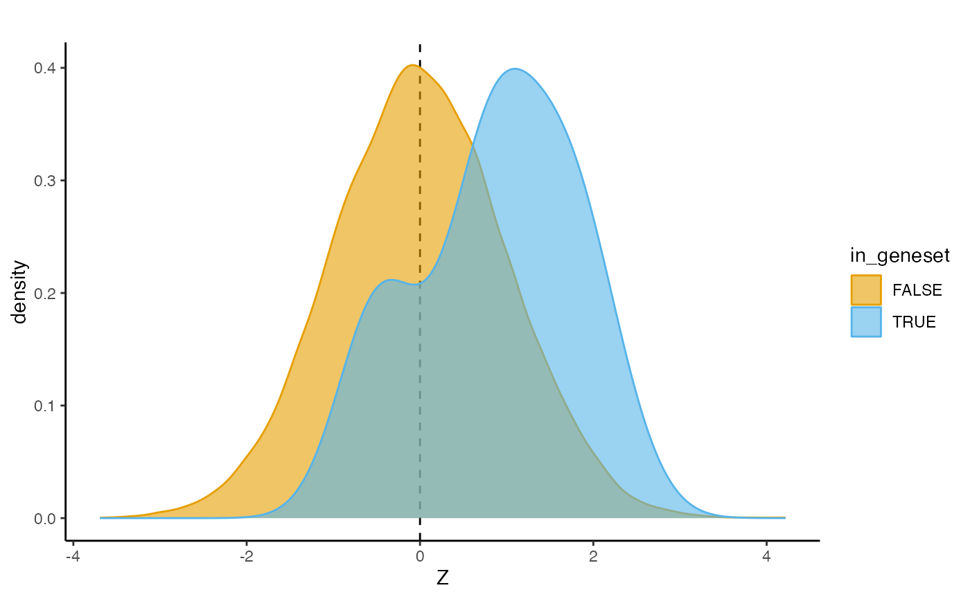

Outlying gene association scores can be remedied by either setting Z-score cutoffs (i.e. all Z-scores exceeding these values will be set to the respective cutoff), or inverse normal transforming the Z-scores:

GSAresults_Zcutoffs <- geneSetAssoc(
  res,
  genesetlist,
  covar = c("nvar"),
  test = c("lm"), 
  minSetSize = 10,
  maxSetSize = 500,
  Zcutoffs = c(-4, 4) # lower and upper bounds
)

GSAresults_INT <- geneSetAssoc(
  res,
  genesetlist,
  covar = c("nvar"),
  test = c("lm"), 
  minSetSize = 10,
  maxSetSize = 500,
  INT = TRUE
)

Conditional gene set analyses can be performed to testher whether gene sets are associated independently with the phenotype of interest. In the example below we condition the most significant geneset on the top 10 most significant genesets. The result includes a condition field, indicating for which gene set the given was adjusted:

topresults <- topResult(GSAresults)
GSAresults_conditional <- geneSetAssoc(
  res,
  getGeneSet(genesetlist, topresults$geneSetName[1]),
  condition = getGeneSet(genesetlist, topresults$geneSetName[2:10]),
  covar = c("nvar"),
  test = c("lm"), 
  minSetSize = 10,
  maxSetSize = 500
)
GSAresults_conditional

## gsaResult with 9 rows and 12 columns
##              geneSetName  test covar threshold geneSetSize  genesObs    effect
##                    <Rle> <Rle> <Rle> <numeric>   <numeric> <numeric> <numeric>
## 1 GOMF_MRNA_METHYLTRAN..    lm  nvar        NA          13        13  0.879184
## 2 GOMF_MRNA_METHYLTRAN..    lm  nvar        NA          13        13  0.879127
## 3 GOMF_MRNA_METHYLTRAN..    lm  nvar        NA          13        13  0.879093
## 4 GOMF_MRNA_METHYLTRAN..    lm  nvar        NA          13        13  0.879132
## 5 GOMF_MRNA_METHYLTRAN..    lm  nvar        NA          13        13  0.879321
## 6 GOMF_MRNA_METHYLTRAN..    lm  nvar        NA          13        13  0.879593
## 7 GOMF_MRNA_METHYLTRAN..    lm  nvar        NA          13        13  0.879231
## 8 GOMF_MRNA_METHYLTRAN..    lm  nvar        NA          13        13  0.879130
## 9 GOMF_MRNA_METHYLTRAN..    lm  nvar        NA          13        13  0.878994
##    effectSE effectCIlower effectCIupper           P              condition
##   <numeric>     <numeric>     <numeric>   <numeric>            <character>
## 1  0.276776      0.423905           Inf 0.000746510       GOMF_BMP_BINDING
## 2  0.276789      0.423826           Inf 0.000747425 GOMF_COA_HYDROLASE_A..
## 3  0.276781      0.423806           Inf 0.000747489 GOMF_DYNEIN_HEAVY_CH..
## 4  0.276781      0.423846           Inf 0.000747119 GOMF_DYNEIN_LIGHT_IN..
## 5  0.276789      0.424021           Inf 0.000745611 GOMF_LIGASE_ACTIVITY..
## 6  0.276788      0.424294           Inf 0.000743074 GOMF_MONOATOMIC_ANIO..
## 7  0.276786      0.423936           Inf 0.000746358 GOMF_PHOSPHATIDYLCHO..
## 8  0.276783      0.423839           Inf 0.000747218 GOMF_PROTEIN_KINASE_..
## 9  0.276784      0.423702           Inf 0.000748516 GOMF_TRANSFERRIN_REC..

Finally, instead of the linear model, a hypergeometric test (test = “fisher”), can be performed if you’d like to tests whether the proportion of P-values below a specified threshold is greater than the proportion outside of it. The threshold parameter specifies the P-value cutoff to define significant genes:

GSAresults_fisher <- geneSetAssoc(
  res,
  genesetlist,
  test = c("fisher"), 
  threshold = 1e-4,
  minSetSize = 10,
  maxSetSize = 500
)
topResult(GSAresults_fisher)

## gsaResult with 10 rows and 11 columns
##               geneSetName   test covar threshold geneSetSize  genesObs
##                     <Rle>  <Rle> <Rle> <numeric>   <numeric> <numeric>
## 1  GOMF_EXTRACELLULAR_M.. fisher    NA     1e-04          10        10
## 2  GOMF_STRUCTURAL_MOLE.. fisher    NA     1e-04          12        12
## 3  GOMF_K63_LINKED_POLY.. fisher    NA     1e-04          26        24
## 4  GOMF_POLYUBIQUITIN_M.. fisher    NA     1e-04          57        52
## 5  GOMF_COPPER_ION_BIND.. fisher    NA     1e-04          63        56
## 6  GOMF_CELL_ADHESION_M.. fisher    NA     1e-04          65        63
## 7  GOMF_ANTIOXIDANT_ACT.. fisher    NA     1e-04          83        80
## 8  GOMF_ATP_DEPENDENT_A.. fisher    NA     1e-04         122       112
## 9  GOMF_PROTEIN_FOLDING.. fisher    NA     1e-04         133       126
## 10 GOMF_PROTEIN_PHOSPHA.. fisher    NA     1e-04         142       138
##       effect  effectSE effectCIlower effectCIupper          P
##    <numeric> <numeric>     <numeric>     <numeric>  <numeric>
## 1   507.6025        NA      18.98856           Inf 0.00271695
## 2   411.5113        NA      15.81130           Inf 0.00325963
## 3   198.1263        NA       7.89375           Inf 0.00651075
## 4    89.4421        NA       3.63563           Inf 0.01406371
## 5    82.9262        NA       3.37545           Inf 0.01513895
## 6    73.7325        NA       2.99909           Inf 0.01701835
## 7    57.7373        NA       2.35945           Inf 0.02157067
## 8    41.0502        NA       1.68226           Inf 0.03009399
## 9    36.4539        NA       1.49414           Inf 0.03380421
## 10   33.2467        NA       1.36333           Inf 0.03697535

Self-contained GSA

Self-contained gene set analyses have been implemented in the form of ‘gene set burden’ analysis.Gene set burden analyses extend the rationale behind gene burden tests to sets of genes, aggregating variants across gene sets rather than single genes. Since this follows the same principle as gene burden testing, the same approach can be used as described in vignette("association_testing"). However, these types of analyses can be computationally demanding since the number of variants to aggregate, especially for large gene sets, is often many times larger than in single gene analyses. Therefore, RVAT also includes an alternative two-step approach. In the first step, burden scores are generated for each gene and stored in a compressed format. In the second step, gene set analyses are performed by aggregating the gene burden scores for each gene set, followed by testing for an association between the gene set burden score and the phenotype of interest. An example of this approach is shown below.

Step 1: generate burden scores per gene

First, we’ll generate a varsetfile, including variants that we want to include in the gene burden scores:

gdb <- gdb(rvat_example("rvatData.gdb"))
buildVarSet(object = gdb, 
            output = paste0(outdir, "/moderate.txt.gz"),
            varSetName = "Moderate", 
            unitTable = "varInfo", 
            unitName = "gene_name",
            where = "ModerateImpact = 1")

Second, burden scores are generated per gene using the aggregate method:

aggregate(x = gdb, 
          varSet=varSetFile(paste0(outdir, "/moderate.txt.gz")),
          maxMAF=0.001,
          output=paste0(outdir, "/moderate.aggregate.txt.gz"),
          verbose = FALSE
          )

Step 2: run gene set burden tests

Note that the example gdb we’re using contains only a small number of genes, therefore most of the genes included in GO, KEGG etc. are missing from this gdb. Therefore, for this example, I’ll just create some dummy genesets that contain genes which are present in the gdb:

varsetfile <- varSetFile(paste0(outdir, "/moderate.txt.gz"))
genesetlist <- buildGeneSet(
  list("geneset1" = listUnits(varsetfile)[c(1,3,4,9)],
       "geneset2" = listUnits(varsetfile)[c(2,4,5,6,10)],
       "geneset3" = listUnits(varsetfile)[c(1,2)],
       "geneset4" = listUnits(varsetfile)[c(7,9,10)],
       "geneset5" = listUnits(varsetfile)))
write(genesetlist,
      file = paste0(outdir, "/genesetfile.txt.gz"))

Perform the gene set burden tests, for this we can use the assocTest method, with the first argument being a aggregateFile connection. Similar to a varSetFile or geneSetFile we can connect to the file containing aggregates (burden scores) using the aggregateFile method:

aggfile <- aggregateFile(paste0(outdir, "/moderate.aggregate.txt.gz"))

We can then run gene set burden tests using the aggregateFile, by passing it as the first argument to assocTest as shown below. Note that, in contrast to running assocTest directly on a genoMatrix or gdb, we cannot perform any variant filters when running assocTest on an aggregateFile. Any variant filters should be applied when generating the aggregates, as shown in step 1.

aggAssoc <- assocTest(
  aggfile,
  gdb = gdb,
  test = c("glm", "firth"),
  cohort = "pheno",
  pheno="pheno",
  geneSet = genesetlist,
  covar = paste0("PC", 1:4),
  verbose = FALSE
)

As noted above, the same results can be obtained by running assocTest directing on a gdb or genoMatrix object, as shown below. However, the two-step approach using is way more more efficient when running large-scale analyses (i.e. ~20,000 genes).

varsetfile <- varSetFile(paste0(outdir, "/moderate.txt.gz"))
units <- listUnits(getGeneSet(genesetlist, "geneset1"))
test <- assocTest(
  object = gdb,
  test = c("glm", "firth"),
  varSet = collapseVarSetList(getVarSet(varsetfile, unit = units), drop = FALSE), # collapse variants across genes into one varSet
  cohort = "pheno",
  pheno="pheno",
  maxMAF=0.001,
  covar = paste0("PC", 1:4),
  verbose = FALSE
)

test

## rvbResult with 2 rows and 24 columns
##          unit cohort varSetName  name pheno           covar geneticModel
##   <character>  <Rle>      <Rle> <Rle> <Rle>           <Rle>        <Rle>
## 1     unnamed  pheno    unnamed  none pheno PC1,PC2,PC3,PC4      allelic
## 2     unnamed  pheno    unnamed  none pheno PC1,PC2,PC3,PC4      allelic
##   MAFweight  test      nvar caseCarriers ctrlCarriers meanCaseScore
##       <Rle> <Rle> <numeric>    <numeric>    <numeric>     <numeric>
## 1         1   glm       543          359         1182     0.0761981
## 2         1 firth       543          359         1182     0.0761981
##   meanCtrlScore     caseN     ctrlN caseCallRate ctrlCallRate    effect
##       <numeric> <numeric> <numeric>    <numeric>    <numeric> <numeric>
## 1     0.0634105      5000     20000      0.96219     0.962038  0.191465
## 2     0.0634105      5000     20000      0.96219     0.962038  0.192340
##    effectSE effectCIlower effectCIupper        OR          P
##   <numeric>     <numeric>     <numeric> <numeric>  <numeric>
## 1 0.0597474     0.0743618      0.308567   1.21102 0.00135265
## 2 0.0596968     0.0741091      0.308223   1.21208 0.00153871

aggAssoc[aggAssoc$geneSetName == "geneset1",]

##   geneSetName cohort name pheno           covar  test geneSetSize genesObs
## 1    geneset1  pheno none pheno PC1,PC2,PC3,PC4   glm           4        4
## 2    geneset1  pheno none pheno PC1,PC2,PC3,PC4 firth           4        4
##   caseN ctrlN meanCaseScore meanCtrlScore    effect   effectSE effectCIlower
## 1  5000 20000    0.07619806    0.06341054 0.1914644 0.05974738    0.07436172
## 2  5000 20000    0.07619806    0.06341054 0.1923395 0.05969681    0.07410904
##   effectCIupper       OR           P
## 1     0.3085671 1.211022 0.001352662
## 2     0.3082229 1.212082 0.001538717

Finally, gene set burden analyses can be run from the command-line, just like other types of assocation tests:

Sys.setenv(rvat = system.file('exec/rvat.R', package = 'rvat'),
           vcfpath = rvatData::rvat_example('rvatData.vcf.gz'),
           phenopath = rvatData::rvat_example('rvatData.pheno'),
           varinfopath = rvatData::rvat_example('rvatData.varinfo'),
           gdbpath = gdb@dbname,
           outdir = outdir)

Rscript $rvat --assocTest \
--gdb $gdbpath \
--geneSet $outdir/genesetfile.txt.gz \
--aggregateFile $outdir/moderate.aggregate.txt.gz \
--name maxMAF001 \
--covar PC1,PC2,PC3,PC4 \
--cohort pheno \
--pheno pheno \
--test glm,firth \
--output $outdir/agg_burden_tests_merged_cmdline.txt.gz

References

Leeuw, Christiaan A. de, Benjamin M. Neale, Tom Heskes, and Danielle Posthuma. 2016. “The Statistical Properties of Gene-Set Analysis.” Nature Reviews Genetics 17 (6): 353–64. https://doi.org/10.1038/nrg.2016.29.