Spatial clustering

library(rvat)
library(rvatData)

This tutorial shows how regional analyses can be performed in RVAT using spatialClust() that is based on an unsupervised approach based on the spatial clustering method by(Loehlein Fier et al. 2017). It partitions variants within genes into consecutive non-overlapping windows. In brief, this algorithm applies a sliding window approach and models the mutation intensity within windows using a non-homogeneous Poisson point process. Within each window variants are then divided at points where the distance is larger than expected under the exponential distribution, thus defining spatially clustered groups of variants.

setup

Initialize gdb and output directory use in this tutorial:

gdb <- create_example_gdb()
outdir <- tempdir()

Map CDS positions

To perform spatial clustering of coding variants, we’ll first map genomic coordinates to CDS coordinates using the mapToCDS method.

# The mapToCds method relies on an ensembl gtf/gff file for remapping 
gtf <- rtracklayer::import("https://ftp.ensembl.org/pub/release-105/gtf/homo_sapiens/Homo_sapiens.GRCh38.105.gtf.gz")

## subset relevant genes
genes <- unique(getAnno(gdb, "varInfo", fields = "gene_name")$gene_name)
gtf <- gtf[gtf$gene_biotype %in% "protein_coding" & 
           gtf$transcript_biotype %in% "protein_coding" & 
           gtf$gene_name %in% genes]

## transcript ids
transcripts <- unique(gtf$transcript_id)

# perform remapping
## note that the `exonPadding` parameter will cause remapping of variants that are 12 base pairs from the exon border to the border.
mapToCDS(
  gdb,
  gff = gtf,
  transcript_id = transcripts,
  exonPadding = 12,
  output = paste0(outdir, "/cdsPOS.txt.gz"),
  biotype = "protein_coding"
)

# upload to gdb
R.utils::gunzip( paste0(outdir, "/cdsPOS.txt.gz"), remove = FALSE, overwrite = TRUE)
uploadAnno(gdb, value = paste0(outdir, "/cdsPOS.txt"), name = "cdsPOS", skipRemap = TRUE)

Perform spatial clustering

Here, we perform spatial clustering for each transcript as described in (Loehlein Fier et al. 2017) and implemented in the spatialClust() method. It is similar to the buildVarSet() method, and will likewise generate a varSetFile. The ‘windowSize’ parameter controls the window size, and the ‘posField` parameter can be used to specify the position field to use, in this case ’cdsPOS’ as generated above.

spatialClust(
  gdb,
  unitTable = "varInfo", 
  varSetName = "ModerateHigh",
  unitName = "transcript_id",
  where = "ModerateImpact = 1 or HighImpact = 1",
  windowSize = 30,
  overlap = 15,
  intersection = "cdsPOS",
  posField = "cdsPOS",
  output = paste0(outdir, "/moderatehigh_clusters.txt.gz")
)

Association testing

Given that spatialClust() generates a varSetFile(), we can as described in other tutorials like the vignette("association_testing") tutorial.

# connect ot the varSetFile
varsetfile <- varSetFile(paste0(outdir, "/moderatehigh_clusters.txt.gz"))

# for this example we'll focus on the ALS gene FUS
units <- listUnits(varsetfile)[stringr::str_detect(listUnits(varsetfile), "ENST00000254108")]

# perform burden tests
burden_spatialclusters <- assocTest(gdb,
                               varSet = getVarSet(varsetfile, unit = units),
                               cohort="pheno",
                               pheno = "pheno",
                               covar = c("sex", "PC1", "PC2", "PC3", "PC4"),
                               test = "firth",
                               name = "spatial_clustering",
                               verbose = FALSE)
burden_spatialclusters

## rvbResult with 5 rows and 24 columns
##                unit cohort         varSetName               name pheno
##         <character>  <Rle>              <Rle>              <Rle> <Rle>
## 1 ENST00000254108_0  pheno ModerateHigh_30_15 spatial_clustering pheno
## 2 ENST00000254108_1  pheno ModerateHigh_30_15 spatial_clustering pheno
## 3 ENST00000254108_2  pheno ModerateHigh_30_15 spatial_clustering pheno
## 4 ENST00000254108_3  pheno ModerateHigh_30_15 spatial_clustering pheno
## 5 ENST00000254108_4  pheno ModerateHigh_30_15 spatial_clustering pheno
##                 covar geneticModel MAFweight  test      nvar caseCarriers
##                 <Rle>        <Rle>     <Rle> <Rle> <numeric>    <numeric>
## 1 sex,PC1,PC2,PC3,PC4      allelic         1 firth        19           15
## 2 sex,PC1,PC2,PC3,PC4      allelic         1 firth         5            1
## 3 sex,PC1,PC2,PC3,PC4      allelic         1 firth         9            2
## 4 sex,PC1,PC2,PC3,PC4      allelic         1 firth         3            1
## 5 sex,PC1,PC2,PC3,PC4      allelic         1 firth        20           18
##   ctrlCarriers meanCaseScore meanCtrlScore     caseN     ctrlN caseCallRate
##      <numeric>     <numeric>     <numeric> <numeric> <numeric>    <numeric>
## 1           44   0.003064461   0.002265313      5000     20000     0.958979
## 2            6   0.000205399   0.000305409      5000     20000     0.978760
## 3           13   0.000416272   0.000666871      5000     20000     0.978400
## 4            2   0.000213562   0.000113819      5000     20000     0.900733
## 5           18   0.003639603   0.000939982      5000     20000     0.971170
##   ctrlCallRate    effect  effectSE effectCIlower effectCIupper        OR
##      <numeric> <numeric> <numeric>     <numeric>     <numeric> <numeric>
## 1     0.958750  0.312226  0.296377     -0.299949      0.870650  1.366463
## 2     0.979250 -0.100711  0.908186     -2.365322      1.464124  0.904195
## 3     0.978533 -0.284614  0.690642     -1.915206      0.912965  0.752304
## 4     0.898733  1.111187  1.033718     -1.281935      3.129786  3.037963
## 5     0.970683  1.444483  0.330752      0.790567      2.098382  4.239660
##             P
##     <numeric>
## 1 3.04661e-01
## 2 9.10852e-01
## 3 6.70675e-01
## 4 3.13982e-01
## 5 2.65621e-05

generate mutation plot

RVAT’s mutationPlot() function provides a convenient way to visualize variants across a gene in a lollipop-plot, while also visualizing additional tracks such as protein domains or mutation clusters as generated above.

prepare data

First, we’ll need to prepare some additional data:
- Single variant statistics to plot along with the spatial clusters.
- Extract cds ranges for spatial clusters (using the getRanges() method). - Retrieve CDS coordinates of the entire transcript.

# perform single variant association tests
sv <- assocTest(gdb,
                varSet = getVarSet(varsetfile, unit = units),
                cohort = "pheno",
                pheno = "pheno",
                covar = c("sex", "PC1", "PC2", "PC3", "PC4"),
                test = "firth",
                name = "sv",
                singlevar = TRUE,
                verbose = FALSE)


# extract CDS ranges for spatial clusters using the `getRanges` method
units <- listUnits(varsetfile)[stringr::str_detect(listUnits(varsetfile), "ENST00000254108")]
varsetlist <- getVarSet(varsetfile, 
                        unit = units)
where <- sprintf("transcript_id = '%s'", stringr::str_split(listUnits(varsetlist), pattern = "_", simplify = TRUE)[,1])
spatialcluster_ranges <- getRanges(
  varsetlist,
  gdb,
  table = "cdsPOS",
  POS = "cdsPOS",
  where = where
)

## add ranges to results
burden_spatialclusters <- merge(
  burden_spatialclusters,
  spatialcluster_ranges[,c("CHROM", "start", "end", "unit")],
  by = "unit"
)

# get CDS positions for single variants
sv_cdsPOS <- getAnno(
  gdb, 
  table = "cdsPOS",
  where = "transcript_id = 'ENST00000254108'"
)
sv_cdsPOS$VAR_id <- as.character(sv_cdsPOS$VAR_id)
sv <- merge(sv, sv_cdsPOS[,c("VAR_id", "cdsPOS")] %>% dplyr::rename(POS = cdsPOS), by = "VAR_id")

# get CDS coordinates using ensembldb
library(ensembldb)
gtf <- gtf[!is.na(gtf$transcript_id) & gtf$transcript_id == "ENST00000254108"]
ensdb_path <- tempfile()
ensdb <- ensembldb::ensDbFromGRanges(
  gtf, 
  outfile = ensdb_path,
  organism = "Homo_sapiens",
  genomeVersion = "GRCh38",
  version = "105"
  )
ensdb <- EnsDb(ensdb_path)

cds <- unlist(genomeToTranscript(sort(gtf[gtf$type == "CDS",]), db = ensdb))
cds <- sort(transcriptToCds(cds, db = ensdb))

generate mutation plot

Generate a mutation plot, including the spatial cluster burden results as a custom track:

plt <- mutationPlot(
  singleVar = sv,
  cds = cds,
  customTracks = burden_spatialclusters
  )
plt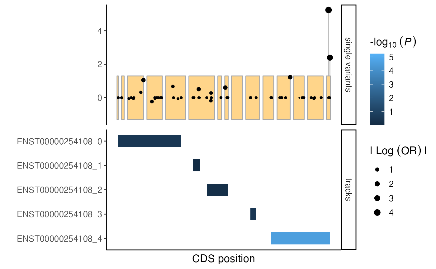

The shapes of the points can be set to indicate the impact of the variant. Below we by visualize moderate impact variants as points and high impact variants by triangles.

# add variant effect predictors to single variant results
varinfo <- getAnno(gdb, "varInfo", VAR_id =  sv$VAR_id)
varinfo$VAR_id <- as.character(varinfo$VAR_id)
varinfo <- varinfo %>%
  dplyr::mutate(
    impact = dplyr::case_when(
      HighImpact == 1 ~ "HIGH",
      ModerateImpact == 1 ~ "MODERATE",
      TRUE ~ NA_character_
    )
  )
sv <- merge(sv, varinfo[,c("VAR_id", "impact")], by = "VAR_id")

# generate mutation plot
plt <- mutationPlot(
  cds = cds,
  customTracks = burden_spatialclusters,
  singleVar = sv,
  impactScale = c("HIGH" = 17, "MODERATE" = 19)
  )
plt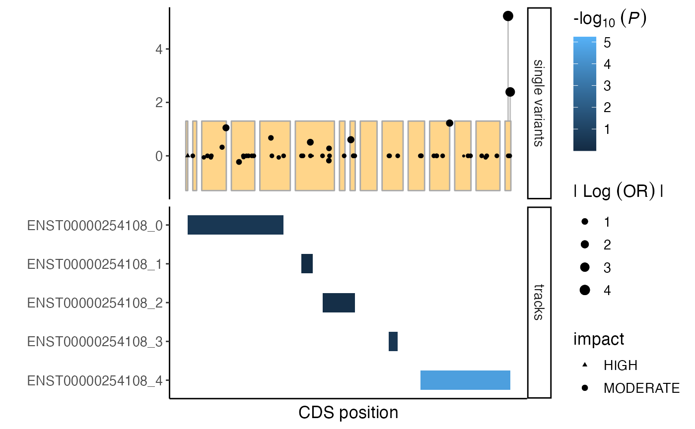

Multiple sets of tracks can be included. In below example we add a whole-gene track. By setting splitByTrackType = TRUE, the spatial cluster and whole gene tracks will be plotted separately. The order of the track types can be set using the trackOrder parameter.

# generate whole-gene test-statistics
burden_wholegene <- assocTest(gdb,
                              VAR_id = sv$VAR_id,
                              cohort = "pheno",
                              pheno = "pheno",
                              covar = c("sex", "PC1", "PC2", "PC3", "PC4"),
                              test = "firth",
                              name = "whole gene",
                              verbose = FALSE)
burden_wholegene$unit <- "ENST00000254108"
burden_wholegene$CHROM <- unique(burden_spatialclusters$CHROM)
burden_wholegene$start <- min(start(cds))
burden_wholegene$end <- max(end(cds))
burden_wholegene$trackType = "gene"
burden_spatialclusters$trackType = "spatial clusters"

# updated custom tracks
tracks <- rbind(burden_wholegene, burden_spatialclusters)

# generate mutation plot
plt <- mutationPlot(
  cds = cds,
  customTracks = tracks,
  singleVar = sv,
  splitByTrackType = TRUE,
  trackOrder = c("gene", "spatial clusters"),
  impactScale = c("HIGH" = 24, "MODERATE" = 21)
  )
plt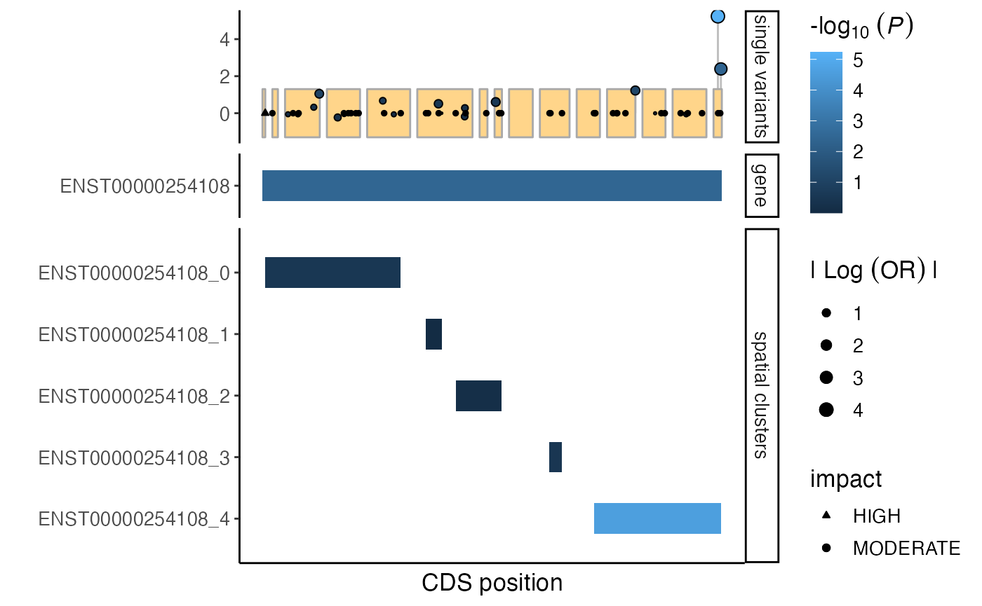

interactive mutation plot

Generate an interactive mutation plot by setting interactive = TRUE. Field to be shown when hovering over elements can be set using the trackHoverFields and svHoverFields parameters.

# round fields that will be shown upon hovering
sv$OR <- signif(sv$OR, 3)
sv$P <- signif(sv$P, 3)
tracks$OR <- signif(tracks$OR, 3)
tracks$P <- signif(tracks$P, 3)

# generate interactive mutation plot
plt <- mutationPlot(
  cds = cds,
  customTracks = tracks,
  singleVar = sv,
  splitByTrackType = TRUE,
  trackOrder = c("gene", "spatial clusters"),
  impactScale = c("HIGH" = 24, "MODERATE" = 21),
  interactive = TRUE,
  trackHoverFields = c("unit", "OR", "P"),
  svHoverFields = c("OR", "P")
  )
plotly::layout(plt, margin = list(l=175))

References

Loehlein Fier, Heide, Dmitry Prokopenko, Julian Hecker, Michael H. Cho, Edwin K. Silverman, Scott T. Weiss, Rudolph E. Tanzi, and Christoph Lange. 2017. “On the Association Analysis of Genome-Sequencing Data: A Spatial Clustering Approach for Partitioning the Entire Genome into Nonoverlapping Windows.” Genetic Epidemiology 41 (4): 332–40. https://doi.org/10.1002/gepi.22040.